CellScan
Analyse cellular signals
Usage
OBJ = CellScan(NAME, RAWIMG, CONFIG, CHANNEL)
Arguments
NAMEis the name for thisCellScanobject.RAWIMGis theRawImgobject that will be used to create theCellScanobject.CONFIGcontains the configuration parameters needed for thecalcFindROIs,calcMeasureROIsandcalcDetectSigsobjects.CHANNELis the channel number to use for analysis.
Details
CellScan objects are used to analyse dynamic fluorescence signals of cellular origin (i.e. calcium dyes and genetic sensors, metabolite sensors, etc.)
See Also
CellScanclass documentationConfigCellScanclass documentationConfigFindROIsDummyclass documentationConfigFindROIsFLIKAclass documentationConfigFindROIsFLIKA_2Dclass documentationConfigFindROIsFLIKA_2p5Dclass documentationConfigFindROIsFLIKA_3Dclass documentationConfigMeasureROIsDummyclass documentationConfigDetectSigsDummyclass documentationConfigDetectSigsClsfyclass documentationCalcFindROIsDummyclass documentationCalcFindROIsFLIKAclass documentationCalcFindROIsFLIKA_2Dclass documentationCalcFindROIsFLIKA_2p5Dclass documentationCalcFindROIsFLIKA_3Dclass documentationCalcMeasureROIsDummyclass documentationCalcDetectSigsDummyclass documentationCalcDetectSigsClsfyclass documentationImgGroupclass documentationImgGroupquick start guide
Examples
The following examples require the sample images and other files, which can be downloaded manually, from the University of Zurich website (http://www.pharma.uzh.ch/en/research/functionalimaging/CHIPS.html), or automatically, by running the function utils.download_example_imgs().
Create a CellScan object interactively
The following example will illustrate the process of creating a CellScan object interactively, starting with calling the constructor.
% Call the CellScan constructor
cs01 = CellScan()
Since no RawImg has been specified, the first stage is to select the type of RawImg to create. Press three and then enter to select the SCIM_Tif.
----- What type of RawImg would you like to load? -----
  >> 1) BioFormats
     2) RawImgDummy
     3) SCIM_Tif
Select a format: 3
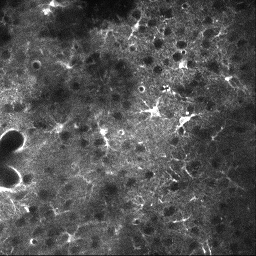
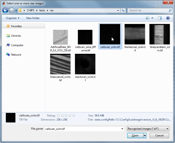
Then, use the interactive dialogue box to select the raw image file cellscan_scim.tif, which should be located in the subfolder tests>res, within the CHIPS root directory.
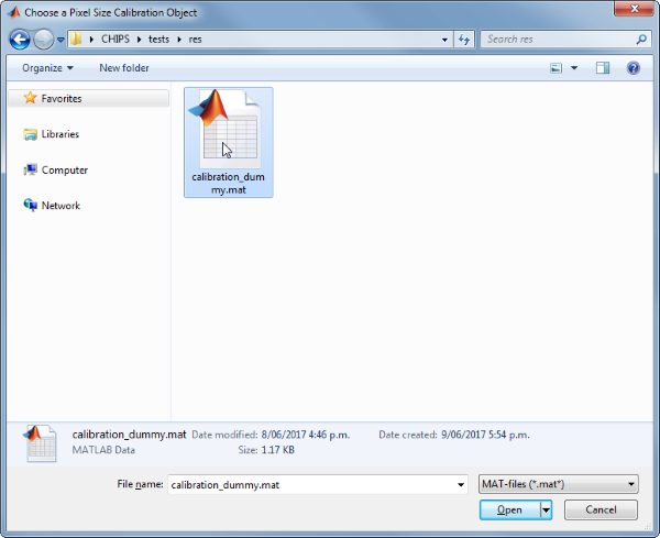
Use the interactive dialogue box to select the dummy calibration (calibration_dummy.mat):
The next stage is to define the ‘meaning’ of the image channel(s). The channel represents a cytosolic calcium sensor in astroytes. Press 1 and then enter to complete the selection.
----- What is shown on channel 1? -----
  >> 0) <blank>
     1) Ca_Cyto_Astro
     2) Ca_Memb_Astro
     3) Ca_Neuron
     4) cellular_signal
     5) FRET_ratio
Answer: 1
Since CellScan objects require a method for ROI identification, a method for ROI measurement, and a method for signal detection, we have to specify our choice.
CellScan defaults to a whole frame analysis (i.e. one ROI covers the whole frame). We’d like to use 3D FLIKA instead, because we want to identify ROIs based on activity. Press 6 and then enter to complete the selection.
----- Which ROI detection method would you like to use? -----
  >> 1) whole frame
     2) load ImageJ ROIs
     3) load mask from .tif or .mat file
     4) 2D FLIKA (automatic ROI selection)
     5) 2.5D FLIKA (automatic ROI selection)
     6) 3D FLIKA (automatic ROI selection)
     7) CellSort (automatic ROI selection)
Select a detection method, please: 6
The next stage is to specify the ROI measuring method. CellScan uses simple baseline calculation as the default. Press enter to complete the selection.
----- Which ROI measuring method would you like to use? -----
>> 1) simple baseline normalised
Select a measuring method, please:
The last stage is to specify the signal detection method. We want to classify signals based on shape and to do some basic measurements like amplitude, etc. Press 2 and then enter to complete the selection.
—– Which signal detection method would you like to use? —–
  >> 1) no signal detection
     2) detect + classify signals
Select a detection method, please: 2
We have now created a CellScan object interactively.
cs01 =
CellScan with properties:
      calcFindROIs: [1x1 CalcFindROIsFLIKA_3D]
   calcMeasureROIs: [1x1 CalcMeasureROIsDummy]
    calcDetectSigs: [1x1 CalcDetectSigsClsfy]
      channelToUse: 1
          plotList: [1x1 struct]
             state: 'unprocessed'
              name: 'cellscan_scim'
            rawImg: [1x1 SCIM_Tif]
The process is almost exactly the same to create an array of CellScan objects; when the software prompts you to select one or more raw images, simply select multiple images by using either the shift or control key.
Prepare a RawImg for use in these examples
% Prepare a rawImg for use in these examples
fnRawImg = fullfile(utils.CHIPS_rootdir, 'tests', 'res', ...
    'cellscan_scim.tif');
channels = struct('Ca_Cyto_Astro', 1);
fnCalibration = fullfile(utils.CHIPS_rootdir, 'tests', 'res', ...
    'calibration_dummy.mat');
calibration = CalibrationPixelSize.load(fnCalibration);
rawImg = SCIM_Tif(fnRawImg, channels, calibration);
Opening cellscan_scim.tif: 100% [==================================]
Create a CellScan object without any interaction
% Create a CellScan object without any interaction
nameCS02 = 'test CS 02';
configFind = ConfigFindROIsFLIKA_3D();
configMeasure = ConfigMeasureROIsDummy();
configDetect = ConfigDetectSigsDummy();
configCS = ConfigCellScan(configFind, configMeasure, configDetect);
channelToUse = 1;
cs02 = CellScan(nameCS02, rawImg, configCS, channelToUse)
cs02 =
  CellScan with properties:

       calcFindROIs: [1×1 CalcFindROIsFLIKA_3D]
    calcMeasureROIs: [1×1 CalcMeasureROIsDummy]
     calcDetectSigs: [1×1 CalcDetectSigsDummy]
       channelToUse: 1
           plotList: [1×1 struct]
              state: 'unprocessed'
               name: 'test CS 02'
             rawImg: [1×1 SCIM_Tif]
Create a CellScan object array
% Create a CellScan object array
rawImgArray(1:3) = copy(rawImg);
rawImgArray = copy(rawImgArray);
csArray = CellScan('test CS Array', rawImgArray, configCS, channelToUse)
csArray =
  1×3 CellScan array with properties:

    calcFindROIs
    calcMeasureROIs
    calcDetectSigs
    channelToUse
    plotList
    state
    name
    rawImg
Create a CellScan object with a custom config
% Create a CellScan object with a custom config
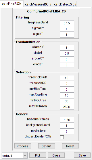
configFindCustom = ConfigFindROIsFLIKA_2D('baselineFrames', 30, ...
'freqPassBand', 0.15, 'sigmaXY', 4, 'dilateXY', 1, ...
'thresholdPuff', 10, 'minRiseTime', 2, 'maxRiseTime', 10, ...
'minROIArea', 36);
configMeasureCustom = ConfigMeasureROIsDummy('baselineFrames', 30);
configDetectCustom = ConfigDetectSigsClsfy('baselineFrames', 30, ...
'thresholdSP', 9, 'lpWindowTime', 6, 'spPassBandMin', 0.015, ...
'spPassBandMax', 0.6, 'spFilterOrder', 10);
configCSCustom = ConfigCellScan(configFindCustom, configMeasureCustom, ...
configDetectCustom);
cs03 = CellScan('test CS 03', rawImg, configCSCustom, channelToUse);
confFind = cs03.calcFindROIs.config
confMeasure = cs03.calcMeasureROIs.config
confDetect = cs03.calcDetectSigs.config
confFind =
  ConfigFindROIsFLIKA_2D with properties:

          threshold2D: 0
       baselineFrames: [30×1 double]
              sigmaXY: 4
               sigmaT: 1
         freqPassBand: 0.1500
        thresholdPuff: 10
          minRiseTime: 2
          maxRiseTime: 10
             dilateXY: 1
              dilateT: 0.5000
              erodeXY: 0
               erodeT: 0
      backgroundLevel: 1
         inpaintIters: 5
    discardBorderROIs: 0
           maxROIArea: 2500
           minROIArea: 36
confMeasure =
  ConfigMeasureROIsDummy with properties:

     baselineFrames: [30×1 double]
    backgroundLevel: 1
      propagateNaNs: 0
confDetect =
  ConfigDetectSigsClsfy with properties:

    backgroundLevel: 1
     baselineFrames: [30×1 double]
        excludeNaNs: 1
       lpWindowTime: 6
      propagateNaNs: 1
      spFilterOrder: 10
      spPassBandMax: 0.6000
      spPassBandMin: 0.0150
        thresholdLP: 7
        thresholdSP: 9
Process a scalar CellScan object
% Process a scalar CellScan object
cs03 = cs03.process()
Finding ROIs: 100% [===============================================]
Measuring ROIs: 100% [=============================================]
Detecting signals: 100% [==========================================]
cs03 =
  CellScan with properties:

       calcFindROIs: [1×1 CalcFindROIsFLIKA_2D]
    calcMeasureROIs: [1×1 CalcMeasureROIsDummy]
     calcDetectSigs: [1×1 CalcDetectSigsClsfy]
       channelToUse: 1
           plotList: [1×1 struct]
              state: 'processed'
               name: 'test CS 03'
             rawImg: [1×1 SCIM_Tif]
Process a CellScan object array (in parallel)
% Process a CellScan object array (in parallel)
% This code requires the Parallel Computing Toolbox to run in parallel
useParallel = true;
csArray = csArray.process(useParallel);
csArray_state = {csArray.state}
Processing array: 100% [===========================================]
csArray_state =
  1×3 cell array
    'processed'    'processed'    'processed'
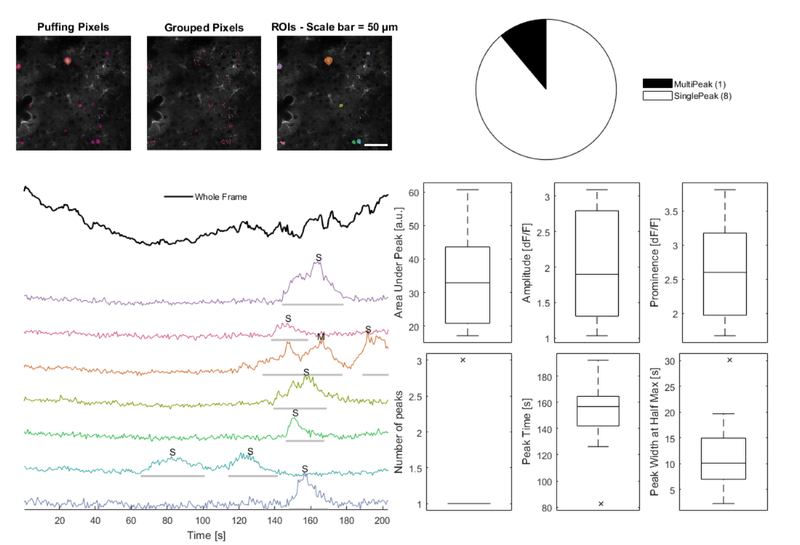
Plot a figure showing an overview of identified ROIs
% Plot a figure showing an overview of identified ROIs
hFig03 = cs03.plot();
set(hFig03, 'Units', 'pixels', 'Position', [50, 50, 1100, 750]);
Produce a GUI to optimise the parameters
% Produce a GUI to optimise the parameters
hFigOpt = cs03.opt_config();
Output the data
% Output the data.  This requires write access to the working directory.
fnCS03 = cs03.output_data('cs03', 'overwrite', true);
% First, the findROIs data
fID03_find = fopen(fnCS03{1}, 'r');
fileContents03f = textscan(fID03_find, '%s');
fileContents03f{1}{1:5}
fclose(fID03_find);
ans =
    'roiNames,area,centroidX,centroidY'
ans =
    'roi0001_0067_0001,112,5.670,69.054'
ans =
    'roi0002_0236_0008,63,13.397,239.286'
ans =
    'roi0003_0053_0107,247,115.061,56.117'
ans =
    'roi0004_0158_0138,50,143.040,156.000'
% Then, the measureROIs data
fID03_measure = fopen(fnCS03{2}, 'r');
fileContents03m = textscan(fID03_measure, '%s');
fileContents03m{1}{1:5}
fclose(fID03_measure);
ans =
    'time,rawTrace,rawTraceNorm,traces_roi0001_0067_0001,traces_roi0002_0236_0008,traces_roi0003_0053_0107,traces_roi0004_0158_0138,traces_roi0005_0236_0168,traces_roi0006_0236_0178,traces_roi0007_0039_0200,tracesNorm_roi0001_0067_0001,tracesNorm_roi0002_0236_0008,tracesNorm_roi0003_0053_0107,tracesNorm_roi0004_0158_0138,tracesNorm_roi0005_0236_0168,tracesNorm_roi0006_0236_0178,tracesNorm_roi0007_0039_0200'
ans =
    '0.339,848.056,0.224,1130.902,1075.889,685.591,1099.540,710.526,934.609,759.978,0.424,0.128,0.071,-0.144,0.312,0.402,0.074'
ans =
    '1.018,863.771,0.345,1126.330,1005.794,727.348,1278.040,656.807,914.379,788.378,0.399,-0.143,0.440,0.514,-0.006,0.307,0.253'
ans =
    '1.696,856.849,0.291,1139.607,1110.540,697.955,1180.100,674.404,841.460,694.978,0.472,0.263,0.180,0.153,0.098,-0.035,-0.334'
ans =
    '2.375,857.652,0.298,1026.821,1076.587,714.008,1161.120,766.965,856.080,765.000,-0.144,0.131,0.322,0.083,0.645,0.034,0.106'
% Finally, the detectSigs data
fID03_detect = fopen(fnCS03{3}, 'r');
fileContents03d = textscan(fID03_detect, '%s');
fileContents03d{1}{1:5}
fclose(fID03_detect);
ans =
    'peakAUC,prominence,amplitude,peakTime,peakStart,peakStartHalf,halfWidth,fullWidth,numPeaks,peakType,roiName'
ans =
    '60.725,3.813,2.294,164.192,144.516,156.729,10.103,33.246,1,SinglePeak,roi0001_0067_0001'
ans =
    '19.096,1.670,1.034,147.230,138.410,140.445,10.921,19.676,1,SinglePeak,roi0002_0236_0008'
ans =
    '17.097,2.970,2.968,192.010,189.296,190.653,2.251,13.570,1,SinglePeak,roi0003_0053_0107'
ans =
    '55.831,2.529,3.090,165.549,133.661,142.481,30.066,43.423,3,MultiPeak,roi0003_0053_0107'