ImgGroup

Contain and analyse groups of processable objects

Usage

OBJ = ImgGroup(RAWIMG, CONFIG, PROCTYPE)
OBJ = ImgGroup(..., PROCOBJ1, PROCOBJ2, ...)
OBJ = ImgGroup(NAME, ...)

Arguments

• RAWIMG is the RawImg object array that will be used to create the ProcessedImg child objects in the ImgGroup object.
• CONFIG is the Config object that will be used to create the ProcessedImg child objects in the ImgGroup object.
• PROCTYPE is the type of ProcessedImg child objects that will be created in the ImgGroup object.
• PROCOBJ1, PROCOBJ2, … are additional ProcessedImg objects that will be added to the ImgGroup object children.
• NAME is the name for this ImgGroup object.

Details

ImgGroup objects are used to contain and analyse groups of processable objects. This can be ProcessedImg objects like LineScanVel or CellScan objects, as well as nested ImgGroup objects.

See Also

• ImgGroup class documentation
• ProcessedImg class documentation
• ProcessedImg quick start guide
• Config class documentation

Examples

The following examples require the sample images and other files, which can be downloaded manually, from the University of Zurich website (http://www.pharma.uzh.ch/en/research/functionalimaging/CHIPS.html), or automatically, by running the function utils.download_example_imgs().

Create an ImgGroup object interactively from one or more files

The following example will illustrate the process of creating a ImgGroup object interactively. Although it is possible to do so by using the constructor method followed by the add() method, it can be easier to use the static method from_files, as illustrated below.

% Construct an ImgGroup using the static method from_files
ig01 = ImgGroup.from_files()

Since no type of ProcessedImg has been specified, the first stage is to specify the type of ProcessedImg to create. Press seven followed by enter to choose a LineScanVel in this case.

----- What type of ProcessableImage would you like to create? -----

  >> 1) ArbLineScan
     2) CellScan
     3) CompositeImg
     4) FrameScan
     5) ImgGroup
     6) LineScanDiam
     7) LineScanVel
     8) MultiChImg
     9) XSectScan

Select a class: 7

Since we are going to choose RawImg files, we must also select the type of RawImg to create. Press three and then enter to select the SCIM_Tif.

----- What type of RawImg would you like to load? -----

  >> 1) BioFormats
     2) RawImgDummy
     3) SCIM_Tif

Select a format: 3

Then, use the interactive dialogue box to select the raw image files framescan_scim.tif and linescanvel_scim.tif (press shift or control/command to select multiple images), which should be located in the subfolder tests>res, within the CHIPS root directory. Although these two images are not really the same type, they will illustrate how to create an ImgGroup object.

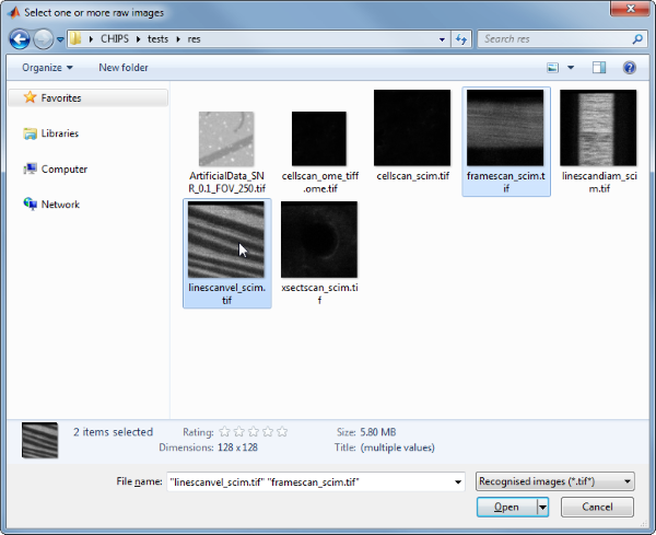
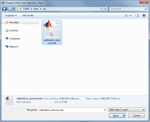
Use the interactive dialogue box to select the dummy calibration (calibration_dummy.mat):

The next stage is to define the ‘meaning’ of the image channels. For this example we will specify the first channel as blood plasma. Press one and enter to complete the selection.

----- What is shown on channel 1? -----

  >> 0) <blank>
     1) blood_plasma
     2) blood_rbcs
     3) Ca_Cyto_Astro
     4) Ca_Memb_Astro
     5) Ca_Neuron
     6) cellular_signal
     7) FRET_ratio

Answer: 1

The next stage is to specify which velocity calculation algorithm should be used. In this case we will choose the Radon transform method. Press two and then enter to complete the selection.

----- What type of velocity calculation would you like to use? -----

  >> 1) CalcVelocityLSPIV
     2) CalcVelocityRadon

Select a format: 2

The final stage is to select the left and right limits of the images to use for velocity calculations. We will not show images here, but the procedure is the same as shown in the LineScanVel examples.

We have now created a ImgGroup object interactively.

ig01 =

ImgGroup with properties:

    children: {[1x1 LineScanVel]  [1x1 LineScanVel]}
   nChildren: 2
       state: 'unprocessed'
        name: []

The process is differerent from creating a LineScanVel object array because the ImgGroup constructor prompts us to choose the left and right limits for velocity calculation for every image, whereas the LineScanVel constructor assumes we want the same limits for every RawImg.

Prepare some RawImg objects for use in these examples

% Prepare a RawImg array for use in these examples
fnRawImgArray = fullfile(utils.CHIPS_rootdir, 'tests', 'res', ...
    'linescanvel_scim.tif');
channelsArray = struct('blood_plasma', 1);
fnCalibration = fullfile(utils.CHIPS_rootdir, 'tests', 'res', ...
    'calibration_dummy.mat');
calibration = CalibrationPixelSize.load(fnCalibration);
rawImgArray(1:2) = SCIM_Tif(fnRawImgArray, channelsArray, calibration);
rawImgArray = copy(rawImgArray)

Opening linescanvel_scim.tif: 100% [===============================]
rawImgArray = 
  1×2 SCIM_Tif array with properties:

    filename
    isDenoised
    isMotionCorrected
    metadata_original
    name
    rawdata
    t0
    metadata

Prepare some ProcessedImg objects for use in these examples

% Prepare a LineScanVel array for use in these examples
nameLSV = 'test LSV';
configRadon = ConfigVelocityRadon('windowTime', 200);
isDarkStreaks = [];
colsToUse = [15 90];
lsvArray = LineScanVel(nameLSV, rawImgArray, configRadon, ...
    isDarkStreaks, colsToUse)

lsvArray = 
  1×2 LineScanVel array with properties:

    plotList
    calcVelocity
    colsToUseVel
    isDarkStreaks
    state
    name
    rawImg

Create an ImgGroup object without any interaction

% Create an ImgGroup object from ProcessedImg objects without any interaction
nameIG02 = 'test IG 02';
ig02 = ImgGroup(nameIG02, lsvArray)

ig02 = 
  ImgGroup with properties:

     children: {[1×2 LineScanVel]}
    nChildren: 1
        state: 'unprocessed'
         name: 'test IG 02'

Add RawImg objects to an existing ImgGroup object with a custom config

% Prepare an extra RawImg for use in this example
fnRawImgXSect = fullfile(utils.CHIPS_rootdir, 'tests', 'res', ...
    'xsectscan_scim.tif');
channelsXSect = struct('blood_plasma', 2);
rawImgXSect = SCIM_Tif(fnRawImgXSect, channelsXSect, calibration);

% Add to an existing ImgGroup object with a custom config
procImgType = 'XSectScan';
configTiRS = ConfigDiameterTiRS('thresholdFWHM', 0.3, ...
    'thresholdInv', 0.25);
ig02.add(rawImgXSect, configTiRS, procImgType);
ig02

Opening xsectscan_scim.tif: 100% [=================================]
ig02 = 
  ImgGroup with properties:

     children: {[1×2 LineScanVel]  [1×1 XSectScan]}
    nChildren: 2
        state: 'unprocessed'
         name: 'test IG 02'

Process an ImgGroup object (in parallel)

% Process an ImgGroup object (in parallel).
% This code requires the Parallel Computing Toolbox to run in parallel
useParallel = true;
ig02 = ig02.process(useParallel)

Processing children: 100% [========================================]
ig02 = 
  ImgGroup with properties:

     children: {[1×2 LineScanVel]  [1×1 XSectScan]}
    nChildren: 2
        state: 'processed'
         name: 'test IG 02'

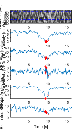
Plot a figure showing the output from all children

% Plot a figure showing the output from all children.
% Note: the figures are deliberately displayed smaller here
hFig = ig02.plot();
set(hFig, 'Position', [50, 50, 300, 500]);

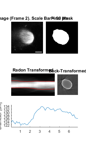
Output the data from all children

% Output the data.  This requires write access to the working directory
fnCSV02 = ig02.output_data('ig02', 'overwrite', true);
fID02 = fopen(fnCSV02{end}{1}, 'r');
fileContents02 = textscan(fID02, '%s');
fileContents02{1}{1:5}
fclose(fID02);

ans =
    'time,diameter,areaPixels,maskSTD,mask'
ans =
    '0.06966,123.58714,2999,FALSE,FALSE'
ans =
    '0.20898,124.89888,3063,FALSE,FALSE'
ans =
    '0.34830,123.64894,3002,FALSE,FALSE'
ans =
    '0.48762,122.57335,2950,FALSE,FALSE'

Home